Main Menu
- Home
- Product Finder
- Calibration Systems
- Calibration Services
- Digital Sensing
- Industrial Vibration Calibration
- Modal and Vibration Testing
- Non-Destructive Testing
- Sound & Vibration Rental Program
- Learn
- About Us
- Contact Us
 Ideal, real world and what’s the difference?
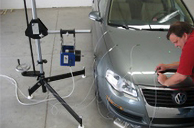
Ever heard the old saying, "No one believes the results of a theoretical analysis except the analyst. And everyone believes the results of an experiment, except the experimentalist"? In the test and measurement world this applies to the fact that vibration sensors are structures just like cars, computers, satellites and machinery that they are used to test. This means that accelerometers undergo stress and show strain, they move, bend, deflect and often show signs of their real world behavior. Test engineers and technicians need to understand the real world behavior of their measurement equipment to ensure that both valid data and valid results are produced.
In the accelerometer world ideal behavior is really quite simple. Ideal accelerometers provide “straight line” behavior. That is to say, a straight-line (linear) relationship for input and output amplitudes, a straight line for FRF magnitude and a straight line for FRF phase. Practically speaking, vendors cannot design or manufacture perfect sensors so there is typically a range where the sensor behavior approximates ideal. This range is often defined as the useful range of the accelerometer in terms of a few of the key specifications; such as amplitude linearity and frequency response.
These key specifications are often governed by electrical or mechanical design choices, but also by the user's choices (such as choice for sensor mounting or discharge time constant of a dynamic signal analyzer’s built in ICP® power). For example, the amplitude linearity is governed by the vendor design choice for the linear range of the internal impedance converting amplifier in an ICP piezoelectric type accelerometer. This is typically expressed as the acceleration “or g-range” that will provide a plus/minus 5 volt swing in the amplifier. In the case of a standard 100 mV/g accelerometer, the amplitude linearity range is plus/minus 50 g’s.
Other key performance specifications rely on the user's choice and action. The frequency response of an accelerometer at higher frequencies is one such spec. Depending on the chosen mounting condition (including surface preparation, choice of adhesive, thickness of adhesive, additional mass of optional mounting hardware like an adhesive mounting base...) all create a family of frequency response curves that are typical of the performance of the mounted sensor.
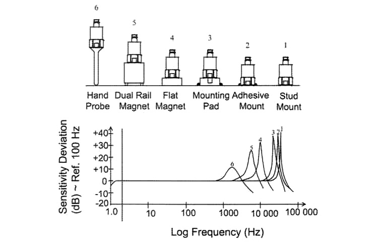
Figure 1 - Effects of Mounting on Resonant Frequency
Typically, the frequency range and sensitivity/resolution of an accelerometer are inversely proportional. As more sensitivity is needed (like seismic monitoring) inertial mass is added to the accelerometer sensing element (which improves sensitivity) and lowers the resonant frequency of the sensing element (and the useful freq range). On the other hand, miniature accelerometers typically have lower sensitivities but extremely high useable frequency ranges. In either case, the real world behavior of the accelerometers approximates a single degree of freedom second order system. This shows the classic frequency response curve like in Figure 2. Note that the useable frequency range in normally described as approximately flat (plus/minus 5% or plus/minus 10% of nominal amplitude sensitivity) and is only about the first 20% of the mounted natural frequency. Curves such as Figure 3 show the effect of sensor damping on the frequency response. In many cases like piezoresistive (PR) and variable capacitance (VC) type accelerometers, critical or near critical damping is desirable to provide a reduced response to higher frequency events like shock or out of band noise.
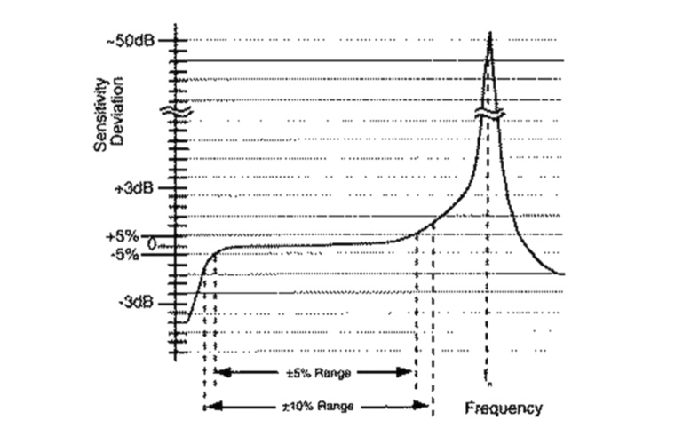 Figure 2 - Frequency Response of Typical ICP® Accelerometers
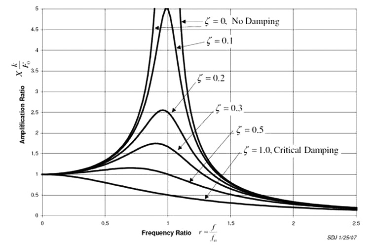
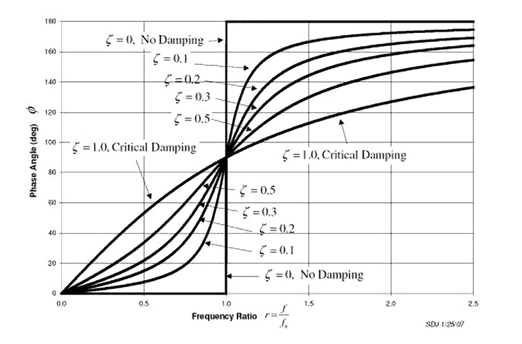
Figure 3 - Effect of Sensor Damping on Frequency Response
A final type of behavior actually depends on both the user's choice and the vendor's design choices. While the discharge time constant of an ICP type accelerometer is fixed (and is critical to ensure adequate low frequency response) the actual response of the measurement channel is determined by the RSS value - the combination of the accelerometer discharge time constant coupled through the discharge time constant of the constant current supply (which can be either a standalone signal conditioner or built-in to the data acquisition / dynamic signal analyzer). To illustrate, consider a modal array type accelerometer useful for structural testing typically has a 1 second discharge time constant which places its ideal 5% roll-off frequency at 0.5 Hz. However, when coupled to an ICP power supply that also has a 1 second discharge time constant, the total measurement channel time constant is calculated by the square root of the sum of the squares, giving a 0.707 discharge time constant. This functionally raises the 5% roll-off frequency to about 0.7 Hz. For AC coupled measurements, a good rule of thumb is to ensure that the signal conditioning discharge time constant is approximately 10x the sensor discharge time constant to provide unaltered low frequency behavior. In cases where extremely low frequency measurement is needed, it is common to switch to DC coupled measurement mode.
In any case, it's best if test engineers and technicians know the real world behavior of their measurement instruments. For the world of accelerometers, it is possible to calibrate and characterize this behavior with simple means like Gravimetric calibration or a more automated approach like a precision accelerometer calibration workstation. Either way, help is just a click or a phone call (513-351-9919) away… we’re glad to help!