Main Menu
- Home
- Product Finder
- Calibration Systems
- Calibration Services
- Digital Sensing
- Industrial Vibration Calibration
- Modal and Vibration Testing
- Non-Destructive Testing
- Sound & Vibration Rental Program
- Learn
- About Us
- Contact Us
In past articles we’ve discussed how interpreting ISO 16063-21 has been a source of confusion when selecting equipment and evaluating measurement uncertainty (Methods for Calibration of Vibration and Shock Transducers; Vibration Calibration by Comparison to a Reference Transducer). This article focuses on one of the most commonly misinterpreted parameters – Total Harmonic Distortion – and its effect on the two most common measurement methodologies.
Distortion is the name given for energy present at any frequency outside of the frequency of interest. In vibration calibration, distortion is often observed in the frequency domain as peaks at frequencies other than the test frequency, typically harmonic in nature.
Distortion can be introduced into a back-to-back calibration through several different means. One of the most common sources of measurement distortion is through non-linearities in the vibration shaker’s centering mechanism – whether this is through mechanical flexures, servo positioning or even rubber support bands. In order to understand and document the uncertainty contribution of distortion on the measurement uncertainty of a back-to-back calibration, the next logical question is: How and when does distortion affect the measurement results themselves?
In back-to-back calibration, we are interested in frequency response of the accelerometer and because of that, the output of the accelerometer should be observed at a single test frequency, stepped over the frequency range of interest. This is typically achieved through one of two different techniques: testing using only a pure sinewave excitation (no distortion) and root mean square (RMS) measurement (time domain), or using a Fourier transform (frequency domain) of the time domain data to isolate the test frequency response from other frequency content. In practice, no mechanical system will produce a 100% distortion-free signal, therefore modern calibration systems will employ the use of a Fourier transform to determine frequency response of a sensor.
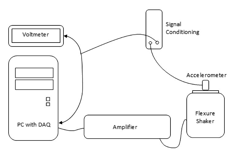
A simple test can be used to illustrate the differences in RMS and Discrete Fourier Transform (DFT) measurements (Figure 1): A mechanical flexure vibration shaker is connected to a power amplifier and signal-generating PC with data acquisition card (DAQ). Affixed to the shaker is an accelerometer which will serve to transduce the vibration signal into a voltage through the signal conditioner. This voltage output will then be fed through a “T” into both the PC’s internal DAQ and an external desktop true RMS voltmeter. The approach for this test will be to observe two signals – one with low distortion, and the other with high distortion – then record measurement results through both RMS and DFT methods. To induce varying levels of distortion, a mechanical flexure shaker is used with test frequencies of 100 Hz (low distortion) and 10 Hz (high distortion). High distortion at 10 Hz is expected with a flexure shaker due to the nature of the mechanical flexures themselves: at high displacement (low frequency), the non-linearity of the flexures will introduce mechanical distortion into the excitation test signal.
The system is run at a 4 g pk level using a 100 Hz test frequency, resulting in a displacement of 0.2 mm (peak to peak). From a visual inspection of the accelerometer’s time waveform, we can see a very clean sine wave with very little distortion (Figure 2).
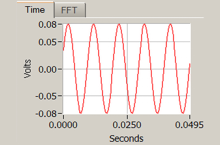
Figure 2: 100 Hz (Low Distortion) Time Domain Signal
From the Fast Fourier Transform we can see the spectral content is relatively small compared to the fundamental frequency. To give a value to the distortion present, the Total Harmonic Distortion (THD) is calculated. THD (%) is the ratio of the summed energy present at harmonic frequencies to the energy present at the fundamental frequency, expressed as a percentage. For this test, THD is computed at 0.1276%.
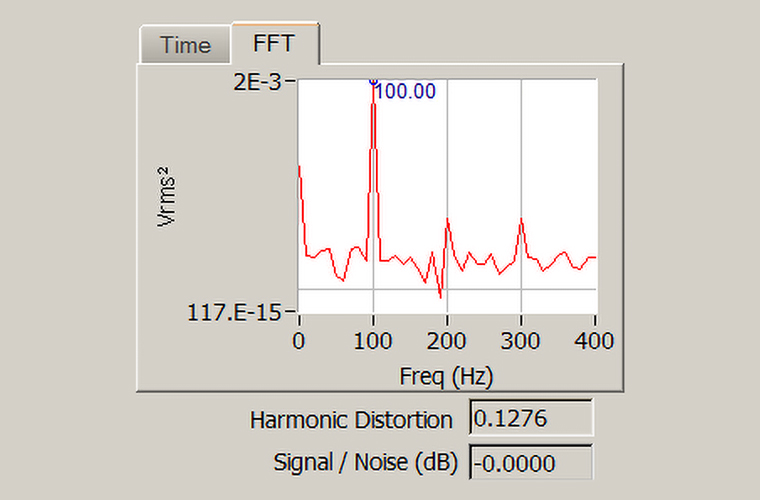
Figure 3: 100 Hz (Low Distortion) Frequency Domain Signal
Repeating this testing again at 4 g pk, using a 10 Hz sine wave, it is easy to visually observe distortion in the time waveform. At this level, the displacement is 20 mm (peak to peak) and begins to show the non-linear effect of the flexures on the sinusoid.
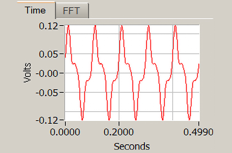
Figure 4: 10 Hz (High Distortion) Time Domain Signal
From the Fast Fourier Transform we can see several harmonic peaks and the THD is computed at 41.1499%.
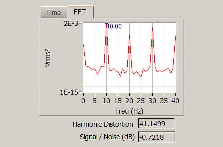
Figure 5: 10 Hz (High Distortion) Frequency Domain Signal
While each measurement plot was recorded, the value of the DFT as read from the DAQ and the value of the RMS voltmeter were recorded. The differences are summarized below.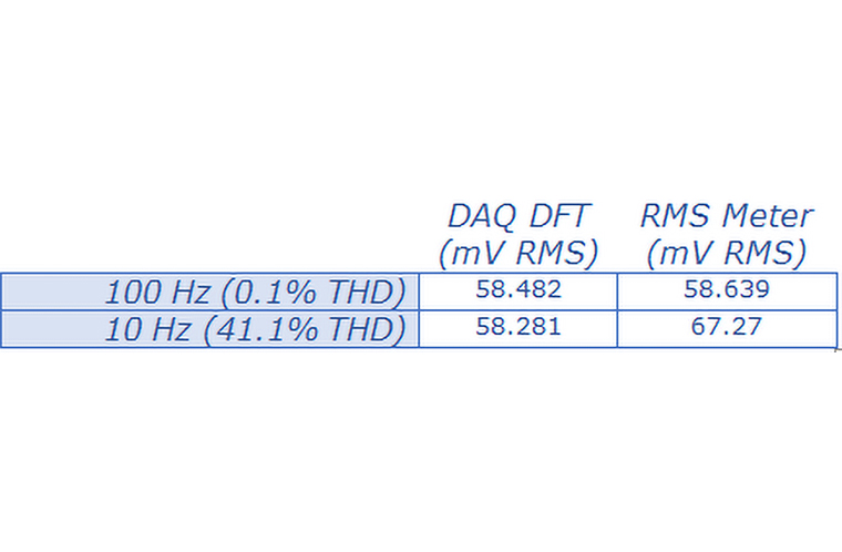
Table 1: Voltage Reading Summary
When we look at the RMS meter output, we can see that there is a dramatic increase (15.4%) of the voltmeter’s RMS value compared to the DAQ’s DFT value. By comparison, the voltmeter’s RMS value is only 0.27% higher for the low distortion (100 Hz) test. This illustrates the superior capability of the Fourier transform: when the distortion in the signal is increased (even vastly so), the voltage reading remains unaffected.
As a result of the differences in these measurement methodologies, the most recent revision of ISO 16063-21:2003(E) addresses their individual implementations. Traditionally, calculating the effect that distortion has on calibration uncertainty when using an RMS method is somewhat complicated. The amount of distortion, dominant harmonic, slope of frequency response for the reference and frequency response slope for the test sensor are all factors influencing the uncertainty analysis. However, ISO 161063-21:2003(E), Section 4.4, Note 1, states that distortion is “normally of no importance” when using narrow band methods such as DFT.
Frequency Response Analyzers utilizing the Fourier transform methodology are “normally preferred instead of broadband RMS voltmeters,” specifically because this measurement technique is insensitive to distortion and eliminates the recommendation for vibration-generating equipment to meet stringent specifications.